Good news here: Google Spreadsheet now support conditional formatting. This post is left here just for nostalgic reasons.

I am a super-heavy user of Google Docs. It is quite amazing what Google made possible with just a simple web browser at hand. I also use Google Spreadsheets a lot, and there was one feature which I was missing a lot: conditional formatting.

No, I’m not talking about the built-in conditional formatting, I’m pretty aware of that one:

 

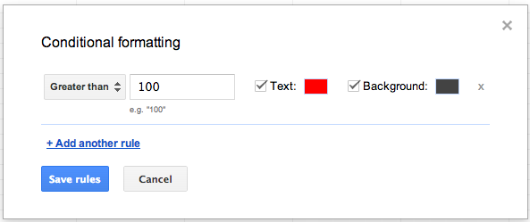
This is pretty straight-forward and simple, and often all you need. But it does not allow you to apply formatting if your task is simple as that: “if the number in cell A is greater than the number in cell B, make the text in cell B appear in red”.

Fortunately, there’s scripting. And scripting in Google Docs is powerful. Have a look at this spreadsheet to get a better understanding what I wanted to accomplish.

 Step 1: Add a script

 

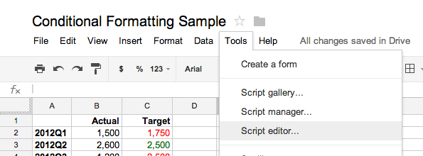
When prompted, I choose “Spreadsheet Project”.

Step 2: Write your function

My function if pretty straight-forward. I wanted to provide it with two ranges. Range 1 is then to be compared with range 2. If the values in range 1 are smaller than in range 2, a certain format should be applied.

function conditionalFormatting(Range1, Range2, targetRange, spreadsheetName, col1, col2)
{
var mySpreadsheet = SpreadsheetApp.getActiveSpreadsheet();
var mySheet = mySpreadsheet.getSheetByName(spreadsheetName);
var range1Values = mySheet.getRange(Range1).getValues();
var range2Values = mySheet.getRange(Range2).getValues();
var target = mySheet.getRange(targetRange);

for (var row in range1Values) {
for (var col in range1Values[row]) {
if (range1Values[row][col] < range2Values[row][col])
mySheet.getRange(target.offset(row, col, 1, 1).getA1Notation()).setFontColor(col1);
else
mySheet.getRange(target.offset(row, col, 1, 1).getA1Notation()).setFontColor(col2);
}
}
}

Step 3: Apply your function!

Later on, I apply my function to two ranges. I use the onEdit-Event that is fired every time a change is made in my spreadsheet:

conditionalFormatting('B2:B5', 'C2:C5', 'C2:C5', 'Sales', 'red', 'green');
conditionalFormatting('B9:B12', 'C9:C12', 'D9:D12', 'Sales', 'red', 'green');

The result is exactly what I wanted:

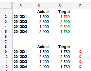
In the upper range, I wanted to colour missed targets with a red font. In the lower range, I wanted to have a separate range that was coloured. Feel free to use the function and alter it to your needs. For example, if you want to colour the background instead of the font, just use the .setBackgroundColor method.